Excel VBA code to compute when a mortgage will be free of PMI (Private Mortgage Insurance)
13 Feb 2020
A friend is trying to come up with a clever way to use Excel to figure out in what month a given mortgage’s principal would have dropped below 80% of the purchase price of the home (at which point they would know longer pay a supplemental fee known as private morgtage insurance, a.k.a. PMI). I didn’t think Excel could do it, but it can.
If you took out a 30-year mortgage at 3.625%, borrowing $225,000 to pay for a $250,000 house, you pay PMI until your principal drops below 80% of $250,000 (that is, until you’ve paid $25,000 of principal).
- (Correction: looks like it’s more like until it drops below 78%. Replace that number in your mind in all my examples below.)
Make a demo custom function
I’m still not sure it can be done in “pure Excel,” but after reading this StackExchange answer, I learned that you can use the programming language built into Excel, VBA, to code your own “functions” that can be used in Excel cells.
It’s pretty slick. Let’s see how to build them and how to use them in spreadsheets.
Build a spreadsheet
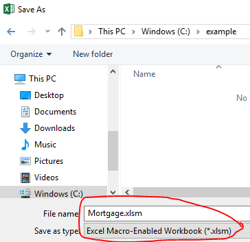
First, make a new Excel file, with the number 0.03625 (that is, 3.625%) in cell B3, and save it in the “.xlsm” filetype (“Excel macro-enabled workbook”).
| A | B | |
|---|---|---|
| 3 | Interest Rate | 0.03625 |
I saved mine at C:\\example\\Mortgage.xlsm.
Add a demo function
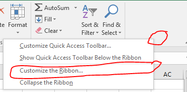
Next, if I don’t already have a “Developer” tab on my “ribbon,” I’ll need to customize the ribbon to add it.
Right-click in the whitespace at the far right edge of the ribbon and click “Customize the Ribbon.”
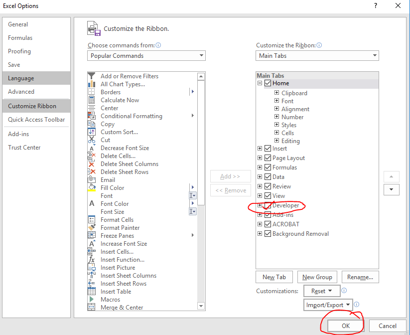
Then check the box next to “Developer” at right if it’s not checked.
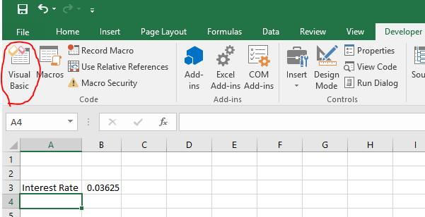
Now click on the “Developer” tab of the ribbon.
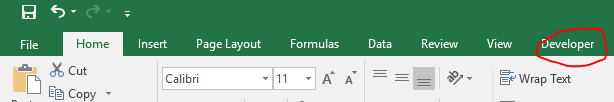
Click the “Visual Basic” button at the far left side of the ribbon.
A new window will pop up. It might look a bit intimidating and programmer-oriented, but this will be easy – I promise.
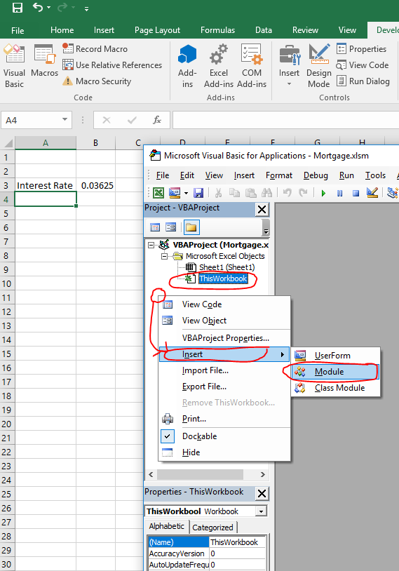
Click on “ThisWorkbook” to select it. It’s under “Microsoft Excel Objects” in the “Project - VBAProject” box in the upper left corner of the screen.
Then right-click in the whitespace below it, still in the “Project - VBAProject” box, and click Insert, followed by Module
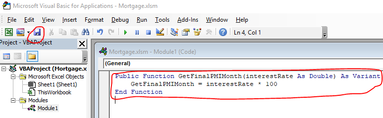
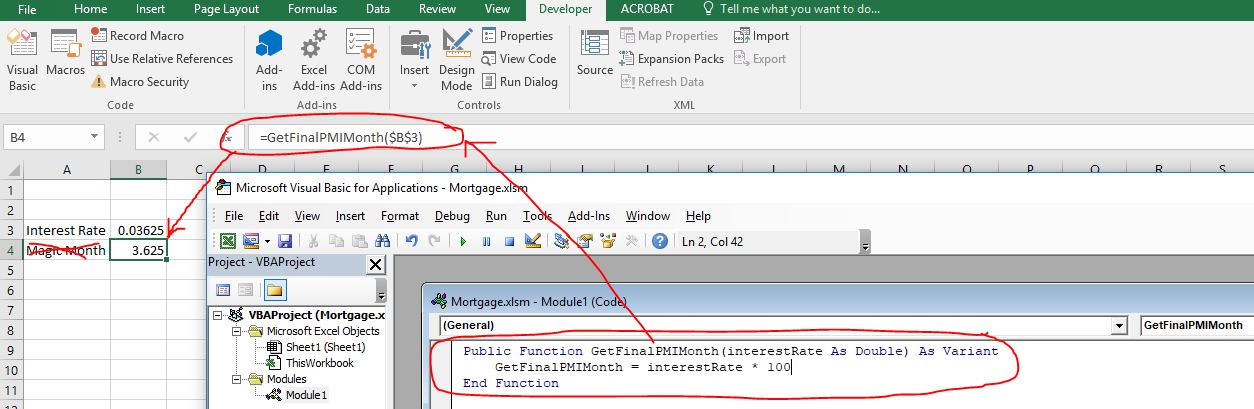
Paste the following code (written in the “VBA” language) into the empty text editor that pops up at right and click the “Save” icon in the upper left part of your screen:
Public Function GetFinalPMIMonth(interestRate As Double) As Variant
    GetFinalPMIMonth = interestRate * 100
End Function
What we’ve just done is add a new “formula” to the list of available formulas that Excel will let us type into a spreadsheet.
We’ve called our formula GetFinalPMIMonth, because eventually, that’s what we’re going to compute with it.
For now, we’ve written the code to insist that anyone who tries to use =GetFinalPMIMonth(...) puts a number (that’s what Double means) into the parentheses. Or a cell reference pointing to a cell that contains a number, anyway.
The last line of the body of our formula definition (which, right now, is the only line), is a bit special.
In repeating the name of the formula itself and putting it on the left-hand side of an equals sign (=), we’re saying that the “output” of the formula should be whatever comes to the right-hand side of the equals sign.
So far, we’re just going to multiply the interest rate by 100 as a proof of concept to demonstrate that we can actually make a custom formula and use it in our spreadsheets.
Hence interestRate * 100 to the right of the =.
Use the demo function
So … let’s give it a try.
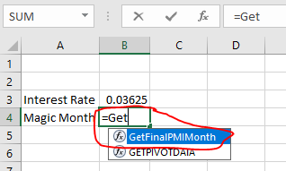
Go back to the window containing your spreadsheet itself and, in cell B4, type =GetFinalPMIMonth(B3) and hit “enter.”
You’ll see that as soon as you get as far as =Get, Excel is suggesting our function. Neat!
Sure enough, the value of cell B4 works out to 3.625.
| A | B | |
|---|---|---|
| 3 | Interest Rate | 0.03625 |
| 4 | 3.625 |
Try editing the value of cell B3 to 0.04 and confirm that B4 updates to 4.
Congratulations – you just wrote your own function for Excel! Great power awaits you.
Make a real custom function
Now we have to make our function a bit more complex.
Build a spreadsheet
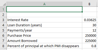
But before we do, let’s put realistic data into our spreadsheet. We’ll fill it out cells A3 through B8 as follows and save our file:
| A | B | |
|---|---|---|
| 3 | Yearly Interest Rate | 0.03625 |
| 4 | Loan Duration (years) | 30 |
| 5 | Payments/year | 12 |
| 6 | Purchase Price | 250000 |
| 7 | Amount Borrowed | 225000 |
| 8 | Percent of principal at which PMI disappears | 0.8 |
(There’s no particular reason I start at A3, besides paranoia that I might later need room for “more stuff” at the top. Start at A1 if you’d like; just adjust your formulas accordingly later on.)
Code the real function
Now we’ll go back to our window with the code editor.
If you accidentally closed it, just click the Developer tab on the ribbon, click Visual Basic, and in the “Modules” folder of the “Project - VBAProject” panel at the top left, double-click “Module1.”
Replace the whole block of code with this, and click the “Save” button in the code-editing window:
Public Function GetFinalPMIMonth( _
    yearlyInterestRate As Double, _
    loanDurationInYears As Integer, _
    paymentsPerYear As Integer, _
    purchasePrice As Double, _
    amountBorrowed As Double, _
    percentAtWhichPMIDisappears As Double _
) As Variant
    'COMMENT: Set up 4 helper variables
    monthlyInterestRate = yearlyInterestRate / paymentsPerYear
    totalPayments = loanDurationInYears * paymentsPerYear
    principalBalanceAtWhichPMIDisappears = purchasePrice * percentAtWhichPMIDisappears
    principalToPayToEliminatePMI = amountBorrowed - principalBalanceAtWhichPMIDisappears
    'COMMENT: Set up loop variables
    whichMonthAreWeAttempting = 1
    principalPaidByEndOfAttemptedMonth = 0
    'COMMENT: Do loop
    While whichMonthAreWeAttempting <= totalPayments And principalPaidByEndOfAttemptedMonth < principalToPayToEliminatePMI
        principalPaidByEndOfAttemptedMonth = -Application.WorksheetFunction.CumPrinc( _
            monthlyInterestRate, _
            totalPayments, _
            amountBorrowed, _
            1, _
            whichMonthAreWeAttempting, _
            0 _
        )
        whichMonthAreWeAttempting = whichMonthAreWeAttempting + 1
    Wend
    'COMMENT: Return output value
    GetFinalPMIMonth = whichMonthAreWeAttempting
End Function
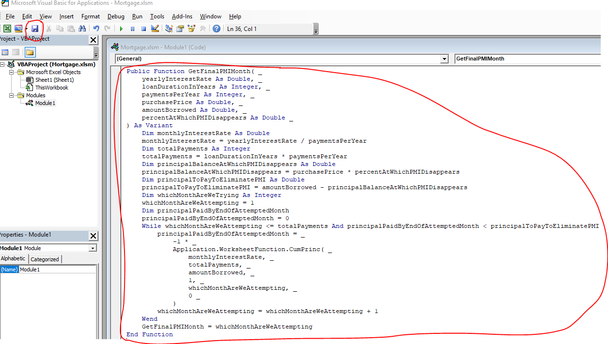
As you can see, our outermost structure still starts with Public function GetFinalPMIMonth( and ends with EndFunction.
I’ll explain the code later in this post – you don’t have to understand it if you’d just like to copy and paste it.
Use the real function
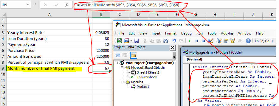
Go back to the window containing your spreadsheet itself and, in cell B9, type =GetFinalPMIMonth(B3, B4, B5, B6, B7, B8) and hit “enter.”
The value of cell B9 works out to 67 months, or about 5 and a half years, just like in my previous example!
Try editing the value of cell B3 to 0.04 and confirm that B9 updates to 70. (That is, it will take you 3 extra months to pay down the principal to $200,000 if your interest rate is 4%).
Does it work? Hooray!
With B3 set back to 0.03625, our final spreadsheet output looks like this now:
| A | B | |
|---|---|---|
| 3 | Yearly Interest Rate | 0.03625 |
| 4 | Loan Duration (years) | 30 |
| 5 | Payments/year | 12 |
| 6 | Purchase Price | 250000 |
| 7 | Amount Borrowed | 225000 |
| 8 | Percent of principal at which PMI disappears | 0.8 |
| 9 | Month number of final PMI payment | 67 |
Further refinements
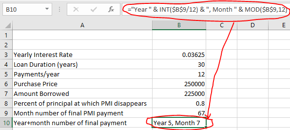
If you’d like one more treat for readability, give yourself an additional formula in B10 that reads ="Year " & INT(B9/12) & ", Month " & MOD(B9,12)
| A | B | |
|---|---|---|
| 10 | Year+month number of final payment | Year 5, Month 7 |
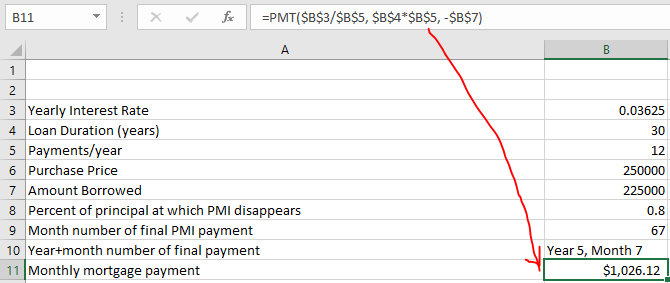
One more thing that might be nice is a quick reference about the monthly mortgage payment we owe the bank in B11: =PMT(B3/B5, B4*B5, -B7) (works out to $1,026.12)
| A | B | |
|---|---|---|
| 11 | Monthly mortgage payment | $1,026.12 |
Door prize - bonus custom functions
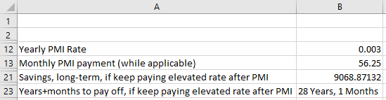
See how much money you would save if you continued to pay your former PMI bill alongside your monthly payment as “extra principal.”
You’l get bonus code for custom functions, plus you’ll see Excel’s CUMIPMT function in action.
Sneak peek:
| A | B | |
|---|---|---|
| 12 | Yearly PMI Rate | 0.003 |
| 13 | Monthly PMI payment (while applicable) | 56.25 |
| 21 | Savings, long-term, if keep paying elevated rate after PMI | $9,068.87 |
| 23 | Years+months to pay off, if keep paying elevated rate after PMI | 28 Years, 1 Months |
Explanation of the code
As promised, for people who like to truly understand what they’re doing, here’s how the VBA I gave you to copy and paste works.
Line breaks
You might note that there are a lot of mysterious places where I ended a line with a single space and an underscore: “ _”
The reason for this is that VBA is a line-break-dependent language. You put one command on each line.
If you are typing a command that is so long you’d have to scroll left and right to read it, you can clarify that adjacent lines should be treated as if they were part of the same line by ending a line with a single space and an underscore.
That’s all that’s going on there.
Input parameters
Note that the number of “input parameters” we’ve written our code to insist users enter got longer. Instead of just 1 called interestRate, we now have 6:
yearlyInterestRate, a number (e.g. “0.03625” as in “3.625%”).loanDurationInYears, an integerpaymentsPerYear, an integerpurchasePrice, a numberamountBorrowed, a numberpercentAtWhichPMIDisappears, a number (e.g. “0.8” as in “80%”)
Helper variables
The meat of our code is in the middle, between As Variant and GetFinalPMIMonth = whichMonthAreWeAttempting.
First, store fixed values into 4 nicknames, or “variable names,” that will be handy in our calculations:
monthlyInterestRate- We’ll set it to the user-provided value of
yearlyInterestRatedivided by the user-provided value ofpaymentsPerYear - Here, that’s
0.03625 / 12, or0.0030208333...
- We’ll set it to the user-provided value of
totalPayments- We’ll set it to the user-provided value of
loanDurationInYearsmultiplied by the user-provided value ofpaymentsPerYear - Here, that’s
360
- We’ll set it to the user-provided value of
principalBalanceAtWhichPMIDisappears- We’ll set it to the user-provided value of
purchasePricemultiplied by the user-provided value ofpercentAtWhichPMIDisappears - Here, that’s
250,000 * 0.8, or200,000
- We’ll set it to the user-provided value of
principalToPayToEliminatePMI- We’ll set it to the value we just computed for
principalBalanceAtWhichPMIDisappearssubtracted from the user-provided value ofamountBorrowed - Here, that’s
225,000 - 200,000, or25,000
- We’ll set it to the value we just computed for
Loop until you get an answer
Next, we set up two more nicknames, or “variable names,” which we will use as scratch-pads, constantly changing their values as we check to see “if we’re there yet”:
whichMonthAreWeAttempting- We’ll start it out saying we’d like to see how much principal we’ll have paid the bank after we finish paying month number
1 - Sneak preview: We’ll constantly increase it by 1 until we’re happy.
- We’ll start it out saying we’d like to see how much principal we’ll have paid the bank after we finish paying month number
principalPaidByEndOfAttemptedMonth- We’ll start it out saying we haven’t yet paid the bank any principal at all (
0) - Sneak preview: We’ll constantly overwrite
principalPaidByEndOfAttemptedMonthwith the output from=CUMPRINC(0.03625/12, 360, 225000, 1, principalPaidByEndOfAttemptedMonth, 0)until we’re happy.
- We’ll start it out saying we haven’t yet paid the bank any principal at all (
Math
I mentioned in my previous post on the subject that mathematically, we’re dealing with a bit of a “calculus problem” – one that involves computing an unknown number based off of known numbers even though “things are changing”.
After all, if you’ve ever looked at an amortization table for a mortgage, you’ve seen that the principal paid is different from one month to the next.
As I recently heard on the radio:
- Algebra is for answering, “If your car is already going 30 miles per hour and holding steady, in how many seconds will you have gone 30 feet?”
- Calculus is for answering, “If your car can accelerate ‘zero miles per hour to sixty miles per hour in 10 seconds,’ in how many seconds will you have gone 30 feet if you ‘floor it’ from a dead stop?”
Cheating
Normally, it’d take a bit more math to calculate the second answer than the first.
But we have an advantage – we don’t pay mortgages in a continuous flow the way a car accelerates. We pay them in monthly lump-sums.
That means we can cheat and avoid a lot of math.
Imagine having your kid in the back seat counting, “One-one-thousand, two-one-thousand, three-one-thousand…” while looking out the window for a big red “30 feet” sign you set out on the side of a racetrack.
(Life pro tip: Do not actually “floor” a car from 0mph to 60mph with your kid in the back seat.)
They’d be able to determine that it was “after two-one-thousand” and “before three-one-thousand,” that they saw the big red sign.
That’s what we’re doing to do with our code here.
- We’re going to try Excel’s
CUMPRINCformula as=CUMPRINC(0.03625/12, 360, 225000, 1, 1, 0)and see whether its value is greater than, or equal to,25,000.- Note that we have to put a minus sign (
-) in front of it becauseCUMPRINCproduces a negative number, and we want a positive number.
- Note that we have to put a minus sign (
- If not, we’ll try the same thing with
=CUMPRINC(0.03625/12, 360, 225000, 1, 2, 0) - If not, we’ll try the same thing with
=CUMPRINC(0.03625/12, 360, 225000, 1, 3, 0) - If not, we’ll try the same thing with
=CUMPRINC(0.03625/12, 360, 225000, 1, 4, 0) - And so on and so forth, quitting as soon as the value is >=
$25,000.
When we get there, we’ll check which number we just punched into the second-to-last parameter of CUMPRINC.
If you’re following along in the code, we’ve been keeping track of this number under the variable name whichMonthAreWeAttempting.
Output value
The value of whichMonthAreWeAttempting when we exit our loop (bounded by While and Wend) is our “magic month” – the final month in which we’ll owe the bank private mortgage insurance on top of our ordinary mortgage payments.
That’s what we want as output for the function, so the final line of the custom function is GetFinalPMIMonth = whichMonthAreWeAttempting.
